Playing the weighting game (I)

In real science images, pixels do not all exhibit identical statistical properties. Some pixels are noisier than others; it may be an intrinsic property, or the result of a gain correction (in vignetted image regions for instance). Some have glitches, are simply unreliable, saturated, or even missing.
Although the FITS standard offers the possibility to tag “bad” pixels (using the BLANK header keyword or NaN image values), it was soon realised that such a description was not adequate enough for processing imaging surveys with variable depth and noise level. Hence came the idea of associating to every science image a weight-map with identical dimensions. The value of a weight-map pixel is an estimate of the precision of the measurement provided by the related science image pixel. This representation has proven to be convenient but is still incomplete. As we shall now see, caution must be taken in using weight-maps.
 |
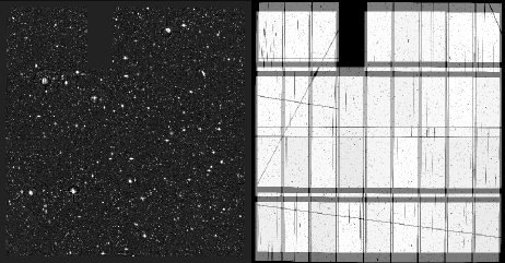
| A stacked image (left) and the associated composite weight-map (right). This was obtained by running SWarp on a set of exposures from the MEGACAM mosaic camera and custom-made weight-maps where bad columns, cosmic-ray impacts, CCD saturation bleeds and satellite trails were give zero weight. The final weight-map provides an accurate chart of the relative background noise level (in terms of inverse variance) to expect in the various parts of the stacked image. From Erben et al. (2009). |
Scaling weights
Weights are most conveniently expressed in units of relative inverse variance:
| $$w_j \propto \frac{1}{\sigma_j^2}$$ | (1) |
A higher weight indicates a lower noise, whereas a weight of 0 translates into infinite variance, and is appropriate for marking a pixel as “bad”. By using relative weights, one can rescale the flux of the science image without having to touch the weight-maps. Software such as SExtractor and SWarp internally calibrate the weight-maps they read and translate them into “absolute” variance maps using a low-resolution noise map derived from the science data themselves. This supposes that the noise process behaves ergodically and that its true variance can be measured at least locally in some parts of the image. The scaling works generally well, but may fail in the most crowded star fields, where no or very little sky background free of objects is available to measure image noise. In those cases a safer approach is to use RMS (root mean square) or variance maps, for which no rescaling is done inside the software.
Handling photon noise
Photon noise is often the main source of noise in modern imagers, and as such has a major influence on the weight-map content. Photon noise follows the Poisson law and variance is proportional to flux. For a sky-noise limited exposure, it may thus sound like a good idea to use the inverse of the image as a weight-map (or the image itself divided by the gain in e–/ADU as a variance map). Noise is seldom stationary because photon flux from bright sources generates additional variance locally. Weight-maps made of image inverses correctly take into account this fact, and could in principle be used to estimate photometric uncertainties, as in SExtractor (we neglect the effect of using “noisy weight-maps” instead of the expected values).
Using weights for combining images
However, such weight-maps would have to be handled with great care if they were to be used for weighted image combination, as in SWarp. As a matter of fact, in SWarp, the weighted combination of N input images can be written as
| $$p’_j=\frac{ \sum_{i\le N} w_{ij} p_{ij}}{\sum_{i \le N} w_{ij}},$$ | (2) |
where $p_{ij}$ and $w_{ij}$ are respectively the value and the weight of image i for pixel j.
The expected flux from the combined data, within an aperture A centred on a source then writes
| $$f_c =E\,(\sum_{j\subset A }p’_j) = E\,\left(\sum_{j\subset A} \frac{\sum_{i\le N} w_{ij} p_{ij}}{\sum_{i\le N} w_{ij}}\right) = \sum_{j\subset A} \frac{\sum_{i\le N} w_{ij} E(p_{ij})}{\sum_{i\le N} w_{ij}},$$ | (3) |
where E () is the expectation operator. Now let’s assume that all input images have the same zero point, and that the aperture A is large enough to contain all the source flux in all images, that is, $\sum_{j\subset A} E(p_{ij}) = f = cste \;\;\forall i$. One easily checks that the weighted combination conserves flux ($f_c=f$) only if
- $w_{ij}$ does not depend on i (input image), or
- $E(p_{ij})$ does not depend on i (same source profile in all input images), or
- $w_{ij}$ does not depend on j (weights are constant within the aperture).
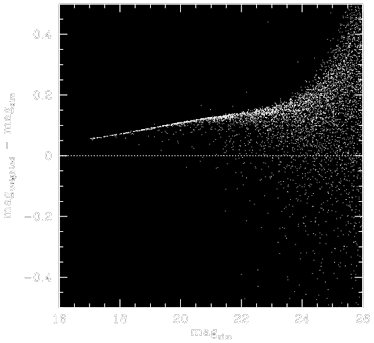
Option (1) weights all input images identically and is therefore useless. (2) only applies in practice if the point-spread function (PSF) is rigorously the same on all images — and if the sky background is also the same or has been subtracted—. Perfectly stable PSFs are seldom seen in practice. Hence unless the PSF has been homogenised on all images we are therefore left with option (3): weight-maps should stay constant within the photometric aperture, or at least in the immediate vicinity of the “cores” of source profiles, where the profile may vary significantly from exposure to exposure. Flux is not conserved in other cases; and using the inverse of input images as weight-maps for instance leads to a strong magnitude-dependent bias in the combined image (illustration below).
 |
Difference between true and recovered stellar aperture magnitude as a function of true magnitude for a weighted combination of 9 simulated images with point-source full-width-at-half-maximum ranging from 2.5 to 5 pixels, when inverse image pixel values are used as weight-maps. Note the strong magnitude-dependent bias. |
This is why AstrOmatic software expects the global envelope of weight or variance maps to concern only the background noise (due to sky background photon statistics and/or read-out noise), as background noise is expected to change little on scale of the seeing disk. For sky background noise-limited images, a flat-field may be used as a weight-map (if there are multiple readout ports, the corresponding image regions should have their gains homogenised first). A weighted combination using these weight-maps is no longer optimal for bright sources, but the degradation should generally be very small in practice; the only case where it is significant is for combinations involving very different exposure times.
Weights in SExtractor
SExtractor uses weight-maps not-only to modulate the detection threshold over the image, but also to estimate measurement uncertainties, for which one can’t afford ignoring the noise from the source photons themselves, at least for bright sources. With “flat” weight-maps, SExtractor has to rely on the image itself, assuming prior knowledge of the gain. For example, the 1-σ uncertainty for a flux measurement in aperture A is computed as:
| $$\sigma_A^2 = \sum_{j\subset A} \left(\sigma_j^2 + \frac{f_j}{g_j}\right),$$ | (4) |
where $\sigma_j^2$ is the variance of the background noise at pixel j derived from the weight-map, $f_j$ the pixel value above the local background (in ADUs), and $g_j$ the pixel gain (in e-/ADU). The user can decide whether the gain $g_j$ should be kept fixed, or if it should be made proportional to the local weight (configuration option WEIGHT_GAIN Y), as when background noise variations are due to flat-field corrections. In that case, it is assumed that the value for the gain in the configuration file or in the image header corresponds to the median weight in the image.
… to be continued (noise correlation, etc.).


4 Comments